Reading a real AUV mission recording
A companion piece to the field guide. That one describes how underwater vehicles organize their data in the abstract; this one opens an actual 377 MB recording from a cave survey and checks whether the patterns hold — and finds four ways the data will quietly mislead you if you take it at face value.
What is actually in the bag
The file is a ROS bag from the Girona Underwater Caves data set: an autonomous vehicle running a sonar and navigation survey inside a flooded cave system. It is 377 MB covering 32.6 minutes, and it holds 661,327 messages across 12 topics.
Before plotting anything, the first job is to ask the recording what it contains. Not what the documentation says it contains — what is in it.
| Topic | Message type | Messages | Hz | Share |
|---|---|---|---|---|
| /tf | tf2_msgs/TFMessage | 249,131 | 127.4 | 37.7% |
| /sonar_seaking | cirs_girona_cala_viuda/RangeImageBeam | 97,501 | 49.9 | 14.7% |
| /sonar_seaking_ros | sensor_msgs/LaserScan | 97,501 | 49.9 | 14.7% |
| /sonar_micron | cirs_girona_cala_viuda/RangeImageBeam | 45,599 | 23.3 | 6.9% |
| /sonar_micron_ros | sensor_msgs/LaserScan | 45,599 | 23.3 | 6.9% |
| /odometry | nav_msgs/Odometry | 21,843 | 11.2 | 3.3% |
| /imu_adis | cirs_girona_cala_viuda/Imu | 19,965 | 10.2 | 3.0% |
| /imu_adis_ros | sensor_msgs/Imu | 19,965 | 10.2 | 3.0% |
| /imu_xsens_mti | cirs_girona_cala_viuda/Imu | 19,553 | 10.0 | 3.0% |
| /imu_xsens_mti_ros | sensor_msgs/Imu | 19,553 | 10.0 | 3.0% |
| /depth_sensor | cirs_girona_cala_viuda/Depth | 19,553 | 10.0 | 3.0% |
| /dvl_linkquest | cirs_girona_cala_viuda/LinkquestDvl | 5,564 | 2.9 | 0.8% |
Two structural things are visible immediately. First, almost every sensor appears twice — once in the manufacturer's own message type and once translated into a ROS standard type. /sonar_seaking and /sonar_seaking_ros carry identical message counts because they are the same pings published two ways. Vendors do this so that standard tooling can consume the data without understanding their proprietary format, at the cost of storing everything twice.
Second, the rates span a wide range. The coordinate-transform topic runs at 127 Hz; the Doppler velocity log runs at 2.9 Hz. That is a 46-fold spread within one vehicle, and it decides what a recording costs to keep.
Where the vehicle went
With the inventory known, the recording can be turned into a picture of the dive. Depth comes from the pressure sensor at 10 Hz; horizontal position comes from the vehicle's own dead-reckoned odometry estimate.
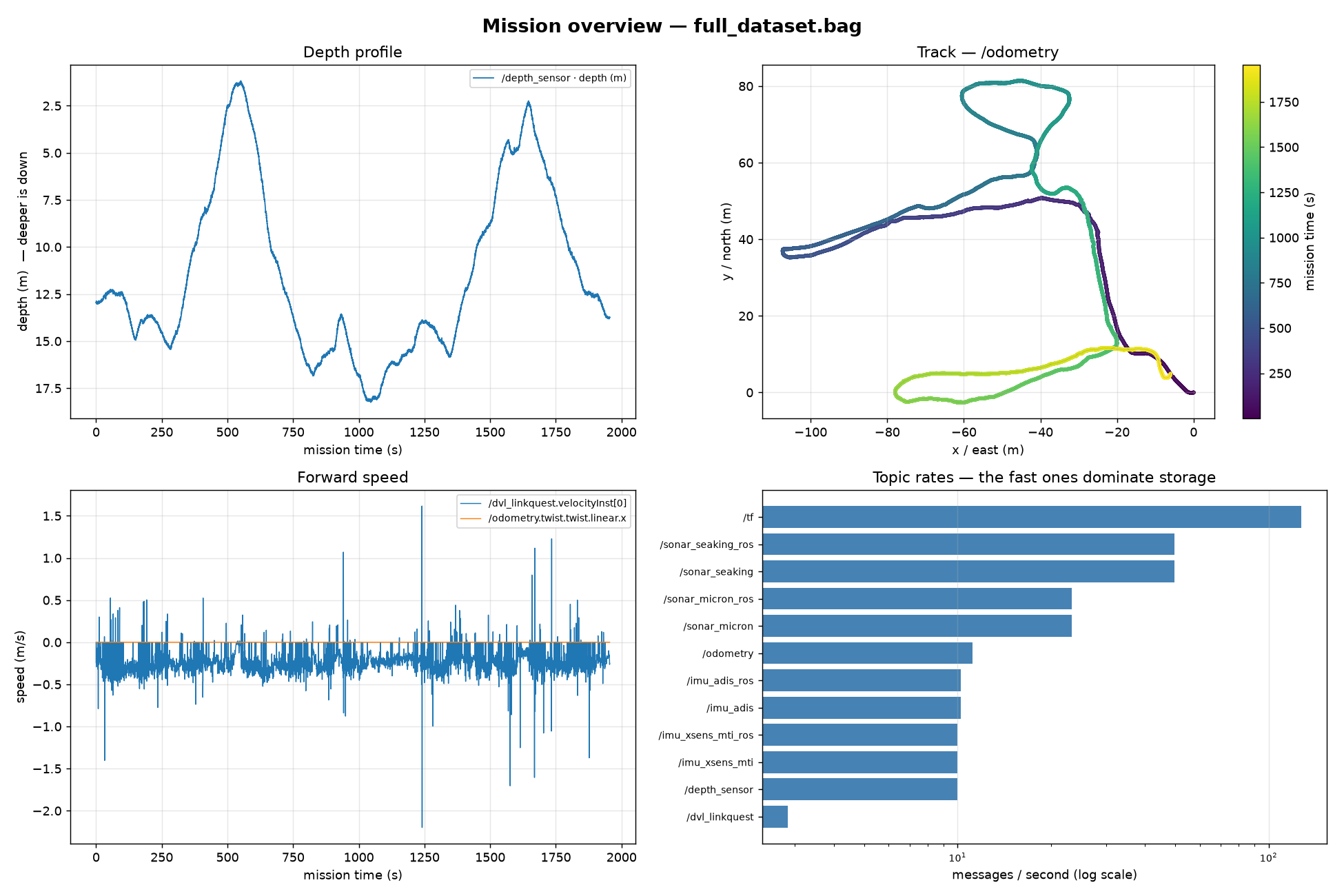
The depth profile and the track together are the whole dive in two pictures, and they are the sanity check everything else rests on. If these look wrong — depth going negative, the track jumping across the map — there is no point analyzing the sonar.
A field that exists but is never filled
The forward-speed panel above has a flat line running through zero. That is not a vehicle sitting still. It is the odometry topic's velocity field, and it is zero for all 21,843 messages.
The nav_msgs/Odometry message has room for both a pose and a twist — where the vehicle is, and how fast it is moving. This recording populates the pose and leaves the twist empty. Nothing in the schema says so; the field is present, correctly typed, and always zero.
A field existing in the message definition does not mean the field carries data. Any speed analysis built on /odometry's twist would have produced a confident, precise, entirely wrong answer of zero. Real speed has to come from the Doppler velocity log instead.
This is worth dwelling on because it is silent. There is no error, no missing topic, no gap in the timeline — just a column of zeros that looks like a measurement.
What the recording is mostly made of
The bottom-right panel is the least visually interesting and the most operationally useful. It ranks every topic by message rate on a log scale, and the ranking is lopsided: /tf, the coordinate-transform tree, is 37.7% of every message in the file.
Coordinate transforms are bookkeeping. They record how the sensor frames relate to the vehicle frame and the world frame — necessary, but not the survey product anyone flew the mission to collect. On this recording, more than a third of the messages are bookkeeping, and the actual Doppler velocity log data is under one percent.
This survey ran 32 minutes. Long-endurance vehicles run for weeks. The rate hierarchy is what decides which topics can be kept at full fidelity, which get downsampled, and which get computed on board and discarded — and that decision is made from exactly this chart, before anyone looks at the science data.
The Doppler velocity log, beam by beam
A Doppler velocity log measures speed over ground by bouncing four acoustic beams off the seafloor and reading the frequency shift on each return. It is how an untethered vehicle knows it is moving when there is no GPS — which, underwater, is always.
Because it depends on getting a usable echo back from four separate directions, it is also the sensor most likely to fail intermittently, and its message carries per-beam detail that makes those failures visible.
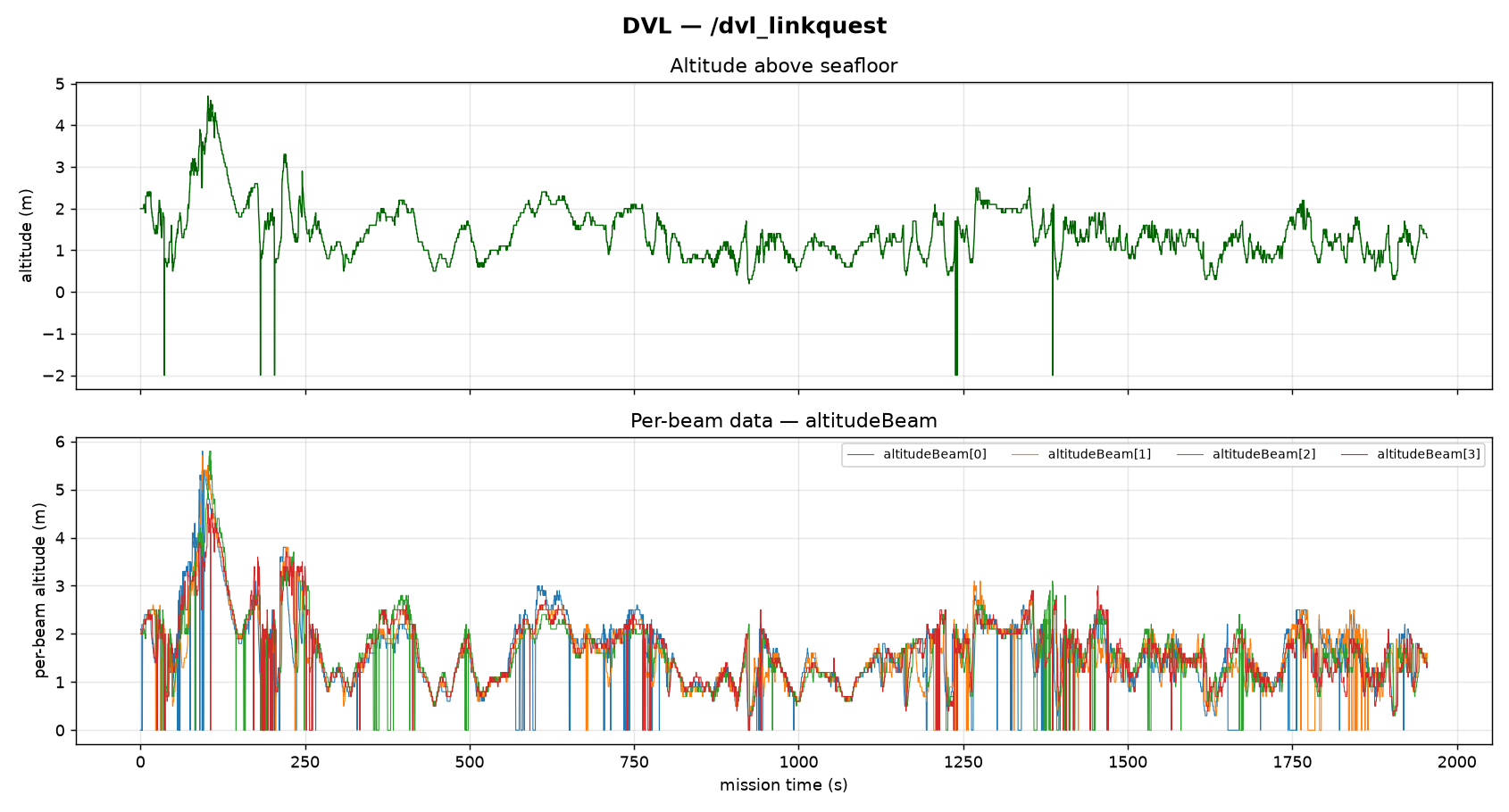
Both panels contain a trap, and they are different traps.
The spikes to −2.0 in the top panel are the instrument's way of saying no bottom lock. Altitude above the seafloor cannot be negative. There are 6 such pings out of 5,564 — only 0.11%, small enough to survive a glance at the summary statistics and large enough to drag a mean in the wrong direction. The same pattern appears in the per-beam data as exactly 0.0.
The message carries a four-element quality flag, one per beam. Reading it shows that only 86.2% of pings have all four beams good. The individual beams are reliable — 94.9%, 97.8%, 95.5% and 98.0% — but the probability that all four succeed at once is much lower than any single beam's reliability suggests. Roughly one ping in seven is degraded.
Neither of these is a defect in the data set. This is what acoustic sensing near a cave wall looks like, and the instrument is reporting its own failures honestly. The failure mode is analytical: both traps are invisible unless the quality flags are read alongside the values, and the flags live in a separate field that a naive extraction would drop.
Which way the vehicle was pointing
The inertial measurement unit reports rotation rate, acceleration, and orientation. This vehicle carries two of them, and — following the pattern from section 01 — each is published both in the manufacturer's format and as a ROS standard message.
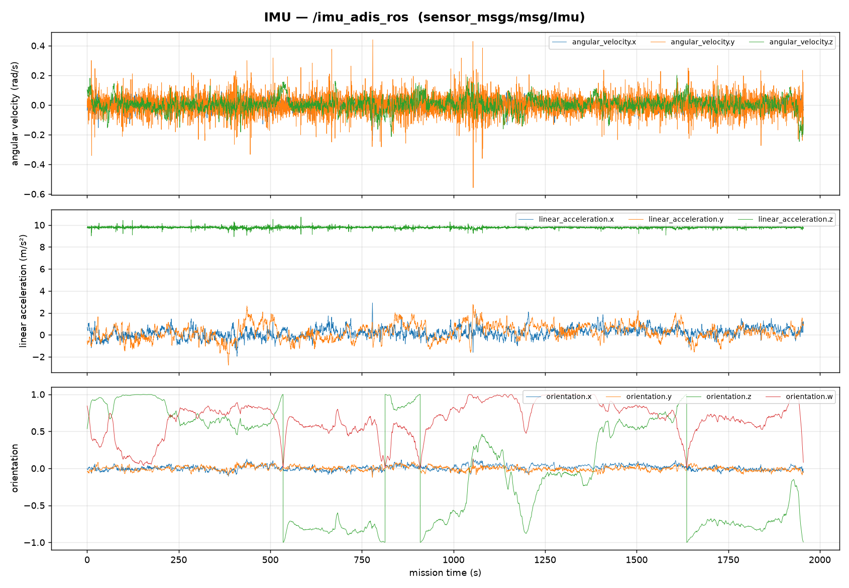
The full-scale vertical jumps in the orientation panel — near t=530, 800, 910 and 1630 s — look like the vehicle instantaneously flipping over. It did not. A quaternion and its exact negative describe the same rotation, so a filter is free to switch between them, and it does. Anything that averages, interpolates, or differentiates these values across a sign flip will produce a violent, entirely fictional rotation.
There is also a practical lesson in which topic produced this figure. The first attempt plotted the manufacturer's IMU message and came back completely blank — the custom type stores the same physics under different field names (gx, ax, roll) than the standard message's nested vectors. The dual-topic pattern from section 01 is not trivia; it determines whether your extraction finds anything at all. When both are present, the standard message is the one to reach for.
How this was done
Everything above was produced on a Windows laptop with no ROS installation. The rosbags library is pure Python and reads both the original ROS bag format and the current one through a single interface, which makes mission data accessible from an ordinary analysis environment — a notebook, a laptop, a container — rather than requiring the robot's own operating system.
One detail makes this possible: the older bag format embeds its message definitions inside the file. The manufacturer-specific types in this recording deserialize correctly without their source packages, because the recording carries its own schema. The bag explains itself.
The working sequence is short. Profile the file to learn its topics, types, and rates. Read one topic at a time into a table, flattening nested message fields into columns and summarizing large arrays rather than exploding them — a sonar ping with thousands of range bins should become a few descriptive statistics, not thousands of columns. Then plot. Profiling the full 377 MB file takes about a second and a half; producing all three figures as well takes about eighteen seconds, most of it drawing rather than reading.
The extraction matches topics by message type rather than by name, so the same code runs unchanged against a different vehicle whose engineers chose different topic names — which is the difference between a script and a tool.
What the four traps have in common
None of them is a corrupted file, a parse error, or a missing topic. Every one of them is well-formed data that means something other than what it appears to mean: a zero that is an absent measurement, a −2 that is an error code, a 0.0 that is a dropped acoustic beam, a sign flip that is not a rotation.
All four survive a schema check. All four survive a plot that nobody looks at closely. They are caught by reading the instrument's own quality flags, knowing what the physical quantity can and cannot do, and treating the sensor's failure reporting as data rather than noise.
That is most of what post-mission analysis actually consists of. The plotting is the easy part.